The Mountain Analogy in ML
2026 Oct 19
See all posts
The mountain/valley analogy is probably the most common pedagogical
tool that people use to explain how models are trained. How far does
that analogy go into modern methods?
The simplest version starts with batch gradient descent on a convex
error surface. Imagine there is only a single weight variable \(w_1\) and some function \(E(w_1)\) which measures the error of the
model given a value for \(w_1\).
"Batch" means that all the training examples are used at once to compute
the error and convex means that \(E\)
has a single global minimum. That global minimum can be thought of as a
valley. We start at a random \(w_1\)
value, which gives us some random error value on all the training
examples. Then we compute the gradient (think direction of steepest
descent) at that random \(w_1\) value
and update \(w_1\) by "taking a step in
that direction." The actual step size is a parameter that we control
called the learning rate. After that one step, we've completed on
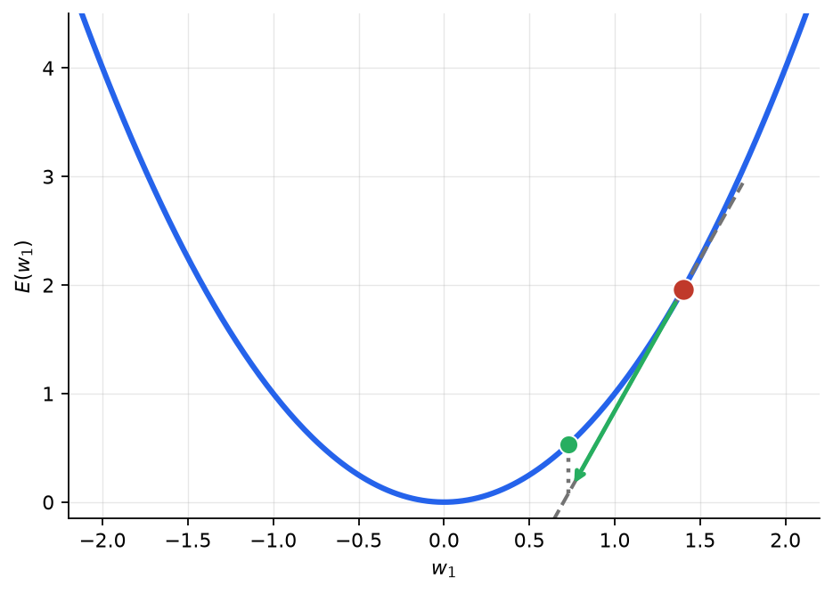
"epoch" worth of training. Visually, what we did was this:
Clearly this isn't guaranteed to get us to the valley. A step size
could be so large that it crosses over the minimum and ends up on the
other side of the valley. However if we make the step size relatively
small and repeat the process over many epochs, we march towards the
valley. When we cross the valley and the error starts rising again, our
direction of steepest descent will point us back towards the valley
again. Smaller steps means more precision in finding the exact lowest
point in the valley, but slower progress.
For models to learn well, they need many more parameters than just a
single \(w_1\) to represent complex
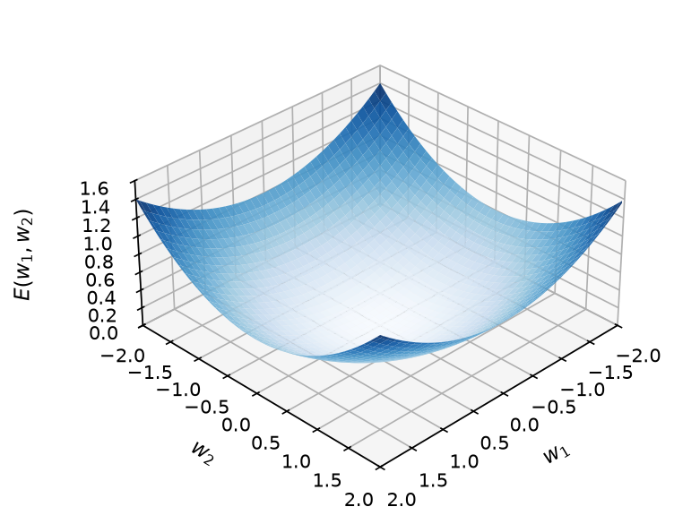
phenomena. Two parameters \(w_1\) and
\(w_2\) can be thought of as a valley
in 3D space:
Adding a 3rd parameter \(w_3\) can
be thought of as making the valley's shape time varying, but with more
parameters it becomes difficult to visualize. In higher dimensions, we
can think of a location as just needing more than \((x,y,z,t)\) to define it, similar to how
your address requires street number, street, city, state, country and so
on. The distance between two locations can still be defined, so a
direction can as well. Taking a step in the direction of steepest
descent still means the same thing, moving as fast as possible towards
the valley.
More parameters means a lot more data because of the curse of
dimensionality, so much so that we often can't practically use all
of the training examples for a single step. Each step must use different
subsets of the total dataset, which is called mini-batch gradient
descent. A batch size of 1 is known as stochastic
gradient descent (SGD). The error surface is defined based on the
training examples, so that means the steps are actually taken on
different error surfaces. The valley is changing shape between every
step. Each batch has its own convex error surface which we take a step
on and our position after that step persists to be re-used as the
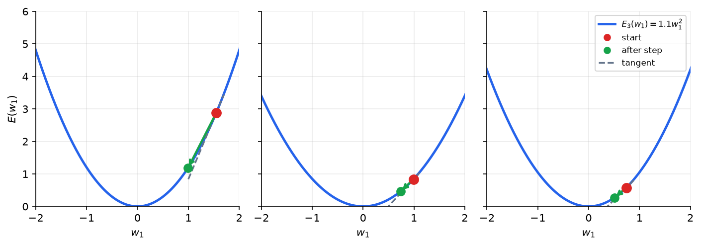
starting point on the next batch's error surface. Consider three steps
with just a single parameter and parabolic convex error surface:
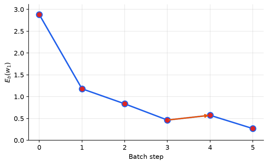
If you were to examine the path taken just in terms of error values,
it might zig zag on its way down because the parameters that yielded the
final position on one mountain might yield a higher position on the next
one.
Mini-batch gradient descent effectively progresses towards the
average valley of a set of valleys corresponding to each batch.
The larger the batch, the more it resembles batch gradient descent. The
smaller the batch, the more zig zagging (noise or jitter) you might do
on your way down. A key reason why mini-batch gradient descent still
works well in practice is that the zig zagging tends to cancel out with
real datasets. If each batch is equally likely to zig or zag, the result
is still a fairly direct route towards the valley average.
What if the error surface is not convex? How does that happen?
Imagine that the output of the model is \(y' = w_1 w_2\) and we measure the loss
as the squared error \(E(w_1, w_2, y) =
(y' - y)^2 = (w_1 w_2 - y)^2\). In that case, the error
surface looks like this:
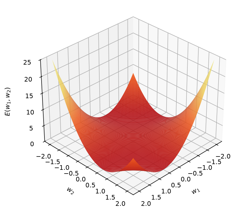
There are now two valleys, which makes sense for any target \(y\) if \(w_1=a\) and \(w_2=b\) is the product that happens to get
close to \(y\) and minimize the error,
\(w_2=a\) and \(w_1=b\) will also be able to do that
because the product will be the same. Models that combine weights in
more complex ways or more complex error computations can result in an
arbitrary number of valleys of arbitrarily different depths. The
fundamental change is that applying batch gradient descent to non-convex
error surfaces will only reach a local valley, which may not be the
lowest valley globally. Furthermore, which local valley you land in
depends on which mountain you start on. The most useful models are
non-convex, so modern ML has developed all kinds of tools to deal with
this multiple valley problem. It turns out that mini-batch gradient
descent already does help to some extent, because when we reset on a
fresh batch with a new mountain its possible that we actually crossed
over some small ridge that we would have gotten caught in without the
mini-batching. One can extend that idea further to doing multiple
training runs from different random start positions and then take the
best result of all of them.
For a messy non-convex error surface, the global minimum may not
necessarily be the best final model. What we really care about is how
well does the model generalize to unseen examples. It will generalize
poorly if the model overfits the training data. Most people intuitively
understand overfitting as something like "using a more complex line than
is required", for example:
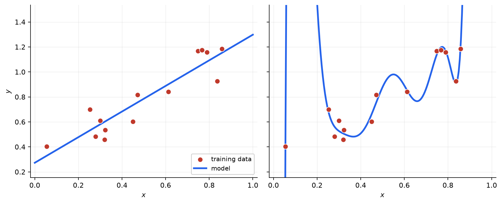
The high degree polynomial stays closer to all the data points so its
error might be lower, but whether or not it fits new data points is
highly variable. In higher dimensional non-convex error surfaces,
"sharp" vs "flat" valleys is a similar idea:
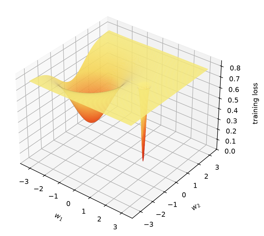
The sharp point might technically have the lowest error value, but it
has high variance. If the unseen data differs even a little bit from the
training data, the error can change significantly. It's more desirable
to find the wide, flat valley where the test data can vary considerably
from the training data and we'll still get low error. The flat valley
casts a wider net, so it can generalize better to diverse test data. How
do you find the wide valleys? Again mini-batch GD potentially helps
"jump over" razor thin valleys because of the zig zag noise it
introduces. That "jumping over" the narrow valleys is really the core
idea behind regularization. It's not so much about finding the wide
valleys as it is avoiding the narrow ones.
Mini-batching isn't the only way to introduce noise that prevents us
from walking down a narrow valley tied to some specific aspect of the
training data. We can change the error surface on every step by
introducing randomness to the network wiring itself. If we randomly
silence different parameters every step, we similarly won't be able to
walk into a narrow valley which requires several steps in a very precise
direction. Instead we'll tend to walk into the wider valleys. That idea
is called "dropout" because parameters randomly drop out from the
network on each step.
Another idea to avoid narrow valleys is to prevent the values of the
parameters from getting too large. Since the parameters are usually
combined with the input via an operation like multiplication, large
parameters effectively increase the variance for the output of the
model. So high weights means the output can swing wildly given small
input changes, creating sharp valleys. If we shrink the weights every
step (weight decay) regardless of the error, we effectively make the
step a 2 part step: one in the direction of steepest descent and a
second one towards the point where all weights are \(0\) (the origin in weight space). This new,
second part of the step effectively gives us little nudges away from
regions where the sharp valleys are more likely to occur.
Aside from regularization, the other challenge that arises in
practice is long and unstable training. Mini-batching introduces zig
zagging and regularization adds computation to each step, both of which
slow down the time it takes to actually find and settle into a valley.
You can think of the zig zagging as if you have a flickering compass.
Naturally, if you were navigating with such a compass, you wouldn't
change your course with every flicker. Not only is that slow but its
unstable - your direction is oscillating. You would take into account
your past heading and only change course when the compass persisted in a
new direction. That is the main idea behind momentum
in ML optimization (see also the older heavy-ball
method) and it is used to improve training speed and stability.
Another source of instability is the fact that so far we've only
discussed constant step sizes. Imagine a mountain descent where some
directions have steep cliffs and others have more gradual descents. If
you took the same step size regardless of the steepness in that
direction, you would have much larger elevation drops in the steep
directions vs the gradual ones. If you continuously did that every step,
you would tend to overcommit to early steep directions and your final
valley would be very sensitive to the starting position. The idea behind
adaptive scaling (optimizers like Adam, AdaGrad, and RMSProp)
is to avoid this by reducing step sizes for these cliff like directions
to improve training stability by dampening initial position
sensitivity.
So you can indeed stretch the mountain/valley analogy all the way to
modern ML, but it strays pretty far from descending a single mountain
via the steepest path down. It's more like: looking for a wide valley in
a shifting mountainous landscape with a biased compass where you adjust
your step size according to incline only change course when the compass
persistently points to a new direction.
Questions or comments? Email feedback@cstein.xyz
The Mountain Analogy in ML
2026 Oct 19 See all postsThe mountain/valley analogy is probably the most common pedagogical tool that people use to explain how models are trained. How far does that analogy go into modern methods?
The simplest version starts with batch gradient descent on a convex error surface. Imagine there is only a single weight variable \(w_1\) and some function \(E(w_1)\) which measures the error of the model given a value for \(w_1\). "Batch" means that all the training examples are used at once to compute the error and convex means that \(E\) has a single global minimum. That global minimum can be thought of as a valley. We start at a random \(w_1\) value, which gives us some random error value on all the training examples. Then we compute the gradient (think direction of steepest descent) at that random \(w_1\) value and update \(w_1\) by "taking a step in that direction." The actual step size is a parameter that we control called the learning rate. After that one step, we've completed on "epoch" worth of training. Visually, what we did was this:
Clearly this isn't guaranteed to get us to the valley. A step size could be so large that it crosses over the minimum and ends up on the other side of the valley. However if we make the step size relatively small and repeat the process over many epochs, we march towards the valley. When we cross the valley and the error starts rising again, our direction of steepest descent will point us back towards the valley again. Smaller steps means more precision in finding the exact lowest point in the valley, but slower progress.
For models to learn well, they need many more parameters than just a single \(w_1\) to represent complex phenomena. Two parameters \(w_1\) and \(w_2\) can be thought of as a valley in 3D space:
Adding a 3rd parameter \(w_3\) can be thought of as making the valley's shape time varying, but with more parameters it becomes difficult to visualize. In higher dimensions, we can think of a location as just needing more than \((x,y,z,t)\) to define it, similar to how your address requires street number, street, city, state, country and so on. The distance between two locations can still be defined, so a direction can as well. Taking a step in the direction of steepest descent still means the same thing, moving as fast as possible towards the valley.
More parameters means a lot more data because of the curse of dimensionality, so much so that we often can't practically use all of the training examples for a single step. Each step must use different subsets of the total dataset, which is called mini-batch gradient descent. A batch size of 1 is known as stochastic gradient descent (SGD). The error surface is defined based on the training examples, so that means the steps are actually taken on different error surfaces. The valley is changing shape between every step. Each batch has its own convex error surface which we take a step on and our position after that step persists to be re-used as the starting point on the next batch's error surface. Consider three steps with just a single parameter and parabolic convex error surface:
If you were to examine the path taken just in terms of error values, it might zig zag on its way down because the parameters that yielded the final position on one mountain might yield a higher position on the next one.
Mini-batch gradient descent effectively progresses towards the average valley of a set of valleys corresponding to each batch. The larger the batch, the more it resembles batch gradient descent. The smaller the batch, the more zig zagging (noise or jitter) you might do on your way down. A key reason why mini-batch gradient descent still works well in practice is that the zig zagging tends to cancel out with real datasets. If each batch is equally likely to zig or zag, the result is still a fairly direct route towards the valley average.
What if the error surface is not convex? How does that happen? Imagine that the output of the model is \(y' = w_1 w_2\) and we measure the loss as the squared error \(E(w_1, w_2, y) = (y' - y)^2 = (w_1 w_2 - y)^2\). In that case, the error surface looks like this:
There are now two valleys, which makes sense for any target \(y\) if \(w_1=a\) and \(w_2=b\) is the product that happens to get close to \(y\) and minimize the error, \(w_2=a\) and \(w_1=b\) will also be able to do that because the product will be the same. Models that combine weights in more complex ways or more complex error computations can result in an arbitrary number of valleys of arbitrarily different depths. The fundamental change is that applying batch gradient descent to non-convex error surfaces will only reach a local valley, which may not be the lowest valley globally. Furthermore, which local valley you land in depends on which mountain you start on. The most useful models are non-convex, so modern ML has developed all kinds of tools to deal with this multiple valley problem. It turns out that mini-batch gradient descent already does help to some extent, because when we reset on a fresh batch with a new mountain its possible that we actually crossed over some small ridge that we would have gotten caught in without the mini-batching. One can extend that idea further to doing multiple training runs from different random start positions and then take the best result of all of them.
For a messy non-convex error surface, the global minimum may not necessarily be the best final model. What we really care about is how well does the model generalize to unseen examples. It will generalize poorly if the model overfits the training data. Most people intuitively understand overfitting as something like "using a more complex line than is required", for example:
The high degree polynomial stays closer to all the data points so its error might be lower, but whether or not it fits new data points is highly variable. In higher dimensional non-convex error surfaces, "sharp" vs "flat" valleys is a similar idea:
The sharp point might technically have the lowest error value, but it has high variance. If the unseen data differs even a little bit from the training data, the error can change significantly. It's more desirable to find the wide, flat valley where the test data can vary considerably from the training data and we'll still get low error. The flat valley casts a wider net, so it can generalize better to diverse test data. How do you find the wide valleys? Again mini-batch GD potentially helps "jump over" razor thin valleys because of the zig zag noise it introduces. That "jumping over" the narrow valleys is really the core idea behind regularization. It's not so much about finding the wide valleys as it is avoiding the narrow ones.
Mini-batching isn't the only way to introduce noise that prevents us from walking down a narrow valley tied to some specific aspect of the training data. We can change the error surface on every step by introducing randomness to the network wiring itself. If we randomly silence different parameters every step, we similarly won't be able to walk into a narrow valley which requires several steps in a very precise direction. Instead we'll tend to walk into the wider valleys. That idea is called "dropout" because parameters randomly drop out from the network on each step.
Another idea to avoid narrow valleys is to prevent the values of the parameters from getting too large. Since the parameters are usually combined with the input via an operation like multiplication, large parameters effectively increase the variance for the output of the model. So high weights means the output can swing wildly given small input changes, creating sharp valleys. If we shrink the weights every step (weight decay) regardless of the error, we effectively make the step a 2 part step: one in the direction of steepest descent and a second one towards the point where all weights are \(0\) (the origin in weight space). This new, second part of the step effectively gives us little nudges away from regions where the sharp valleys are more likely to occur.
Aside from regularization, the other challenge that arises in practice is long and unstable training. Mini-batching introduces zig zagging and regularization adds computation to each step, both of which slow down the time it takes to actually find and settle into a valley. You can think of the zig zagging as if you have a flickering compass. Naturally, if you were navigating with such a compass, you wouldn't change your course with every flicker. Not only is that slow but its unstable - your direction is oscillating. You would take into account your past heading and only change course when the compass persisted in a new direction. That is the main idea behind momentum in ML optimization (see also the older heavy-ball method) and it is used to improve training speed and stability. Another source of instability is the fact that so far we've only discussed constant step sizes. Imagine a mountain descent where some directions have steep cliffs and others have more gradual descents. If you took the same step size regardless of the steepness in that direction, you would have much larger elevation drops in the steep directions vs the gradual ones. If you continuously did that every step, you would tend to overcommit to early steep directions and your final valley would be very sensitive to the starting position. The idea behind adaptive scaling (optimizers like Adam, AdaGrad, and RMSProp) is to avoid this by reducing step sizes for these cliff like directions to improve training stability by dampening initial position sensitivity.
So you can indeed stretch the mountain/valley analogy all the way to modern ML, but it strays pretty far from descending a single mountain via the steepest path down. It's more like: looking for a wide valley in a shifting mountainous landscape with a biased compass where you adjust your step size according to incline only change course when the compass persistently points to a new direction.
Questions or comments? Email feedback@cstein.xyz